Diffusion modeling

DATA_PATH

PosixPath('/home/runner/work/nipreps-book/nipreps-book/data/dwi_full_brainmask.h5')

The proposed method requires inferring a motion-less, reference DW map for a given diffusion orientation for which we want to estimate the misalignment. Inference of the reference map is achieved by first fitting some diffusion model (which we will draw from DIPY) using all data, except the particular DW map that is to be aligned. We will be using the nifreeze.data.splitting.lovo_split utility (LOVO = leave one volume out), that basically leverages the indexing feature of our data structure to partition the dataset into test and train.

All models are required to offer the same API (application programmer interface):

1. The initialization takes a DIPY GradientTable as the first argument, and then arbitrary parameters as keyword arguments.

2. A fit(data) method, which only requires a positional argument data, a 4D array with DWI data.

3. A predict(gradient_table) method, which only requires a GradientTable as input. This method produces a prediction of the signal for every voxel in every direction represented in the input gradient_table.

Attention

By default, the code running in each Jupyter notebook is its own process. We must reload the dataset again to use it in this notebook.

from nifreeze.data.dmri import DWI
from nifreeze.data.splitting import lovo_split
from nireports.reportlets.modality.dwi import plot_dwi

dmri_dataset = DWI.from_filename(DATA_PATH)

Implementing a trivial model

We will first start implementing a trivial model. This model will always return the reference b=0 map, regardless of the particular diffusion orientation model. In other words, it is just a constant model.

Its simplicity does not diminish its great usefulness. First, when coding it is very important to build up iteratively in complexity. This model will allow to easily test the overall integration of the different components of our head-motion estimation algorithm. Also, this model will allow a very straightforward implementation of registration to the b=0 reference, which is commonly used to initialize the head-motion estimation parameters.

class TrivialB0Model:
    """
    A trivial model that returns a *b=0* map always.

    Implements the interface of :obj:`dipy.reconst.base.ReconstModel`.
    Instead of inheriting from the abstract base, this implementation
    follows type adaptation principles, as it is easier to maintain
    and to read (see https://www.youtube.com/watch?v=3MNVP9-hglc).

    """

    __slots__ = ("_S0",)

    def __init__(self, gtab, S0=None, **kwargs):
        """Implement object initialization."""
        if S0 is None:
            raise ValueError("S0 must be provided")

        self._S0 = S0

    def fit(self, *args, **kwargs):
        """Do nothing."""

    def predict(self, gradient, **kwargs):
        """Return the *b=0* map."""
        return self._S0

The model can easily be initialized as follows (assuming we still have our dataset loaded):

model = TrivialB0Model(
    dmri_dataset.gradients,
    S0=dmri_dataset.bzero,
)

Then, at each iteration of our estimation strategy, we will fit this model to the data, after holding one particular direction (data_test) out, using the lovo_split utility. In every iteration, this finds the b=0 volumes in the data and averages their values in every voxel:

data_train, data_test = lovo_split(dmri_dataset, 5)
model.fit(np.squeeze(data_train[0]))

Finally, we can generate our registration reference with the predict() method:

predict_b = np.squeeze(data_test[2])
predicted = model.predict(predict_b)
plot_dwi(predicted, dmri_dataset.affine, gradient=predict_b);

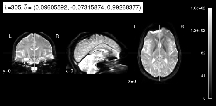
As expected, the b=0 doesn’t look very much like the particular left-out direction, but it is a start!

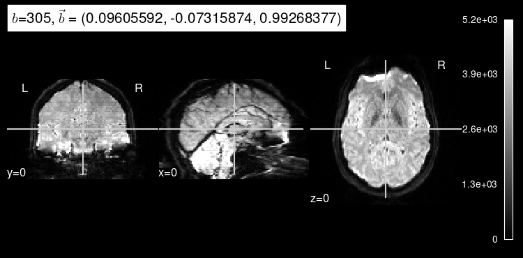
plot_dwi(np.squeeze(data_test[0]), dmri_dataset.affine, gradient=predict_b);

Implementing a regression to the mean model

Exercise

Extend the TrivialB0Model to produce an average of all other diffusion directions, instead of the b=0.

class AverageDWModel:
    """A trivial model that returns an average map."""

    __slots__ = ("_data",)

    def __init__(self, gtab, **kwargs):
        """Implement object initialization."""
        return  # do nothing at initialization time

    def fit(self, data, **kwargs):
        """Calculate the average."""
        # self._data =  # Use numpy to calculate the average.

    def predict(self, gradient, **kwargs):
        """Return the average map."""
        return self._data

Solution

Show code cell content

Hide code cell content

class AverageDWModel:
    """A trivial model that returns an average map."""

    __slots__ = ("_data",)

    def __init__(self, gtab, **kwargs):
        """Implement object initialization."""
        return  # do nothing at initialization time

    def fit(self, data, **kwargs):
        """Calculate the average."""
        self._data =  data.mean(-1)

    def predict(self, gradient, **kwargs):
        """Return the average map."""
        return self._data

Exercise

Use the new AverageDWModel you just created.

Solution

Show code cell content

Hide code cell content

model = AverageDWModel(
    dmri_dataset.gradients,
)
model.fit(data_train[0])
predicted = model.predict(data_test[1])
plot_dwi(predicted, dmri_dataset.affine, gradient=predict_b);
plot_dwi(np.squeeze(data_test[0]), dmri_dataset.affine, gradient=predict_b);

Investigating the tensor model

Now, we are ready to use the diffusion tensor model. We will use the wrap around DIPY’s implementation that we distribute with nifreeze.

The model factory

To permit flexibility in selecting models, the nifreeze package offers a ModelFactory that implements the facade design pattern. This means that ModelFactory makes it easier for the user to switch between models:

from nifreeze.model import ModelFactory

model = ModelFactory.init(
    dataset=dmri_dataset,
    model="DTI",
)

Leveraging the fit() / predict() API

The ModelFactory returns a model object that is compliant with the interface sketched above:

predicted = model.fit_predict(88, n_jobs=16)

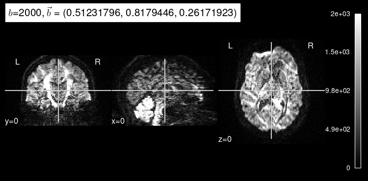
Now, the predicted map for the particular b gradient looks much closer to the original:

plot_dwi(predicted, dmri_dataset.affine, gradient=test_b, black_bg=True);

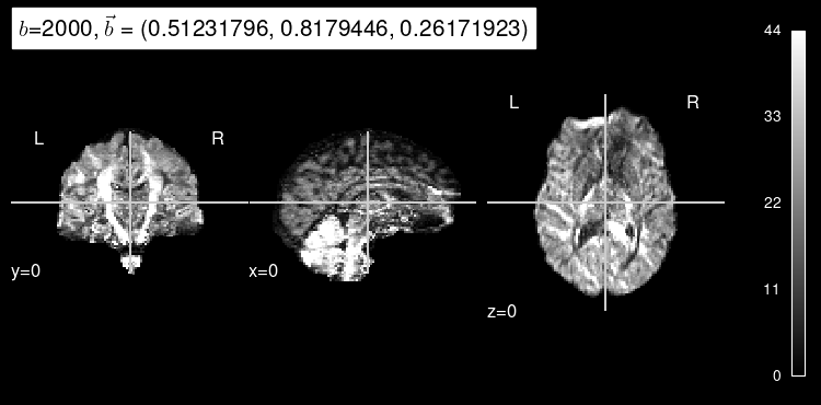
Here’s the original DW map, for reference:

plot_dwi(test_data, dmri_dataset.affine, gradient=test_b);

Exercise

Use the ModelFactory to initialize a "DKI" (diffusion Kurtosis imaging) model.

Solution

Show code cell content

Hide code cell content

model = ModelFactory.init(
    dataset=dmri_dataset,
    model="DKI",
)

Once the model has been initialized, we can easily generate a new prediction.

predicted = model.fit_predict(88, n_jobs=16)
plot_dwi(predicted, dmri_dataset.affine, gradient=test_b, black_bg=True);
plot_dwi(test_data, dmri_dataset.affine, gradient=test_b);

Next steps: image registration

Once we have our model factory readily available, it will be easy to generate predictions that we can use for reference in image registration.