Image registration (spatial alignment)#
At this point of the tutorial we have covered two of the three initial requirements:
we have a powerful data structure to access our dMRI dataset with agility, and
we have a reliable (thanks to DIPY!) model factory to generate motion-less references.
Therefore, we are only one step away from our goal - aligning any given DW map with the motion-less reference. The estimation of the spatial transform that brings two maps into alignment is called image registration.
Image registration is therefore the process through which we bring the structural features of two images into alignment. This means that, brain sulci and gyri, the ventricles, subcortical structures, etc. are located exactly at the same place in the two images. That allows, for instance, for image fusion, and hence screening both images together (for example, applying some transparency to the one on top) should not give us the perception that they are not aligned.
ANTs - Advanced Normalization ToolS#
The ANTs toolbox is widely recognized as a powerful image registration (and normalization, which is registration to some standard space) framework.
The output of an image registration process is the estimated transform that brings the information in the two images into alignment. In our case, the head-motion is a rigid-body displacement of the head. Therefore, a very simple (linear) model –an affine \(4\times 4\) matrix– can be used to formalize the estimated transforms.
Only very recently, ANTs offers a Python interface to run their tools. For this reason, we will use the very much consolidated Nipype wrapping of the ANTs’ command-line interface. The code is almost as simple as follows:
from nipype.interfaces.ants import Registration

registration_framework = Registration(
    fixed_image="reference.nii.gz",
    moving_image="left-out-gradient.nii.gz",
    from_file="settings-file.json"
)
At the minimum, we need to establish our registration framework using the fixed (our synthetic, motion-less reference) and the moving (the left-out gradient) images.
We can easily configure registration by creating a settings-file.json that may look like the following:
{
  "collapse_output_transforms": true,
  "convergence_threshold": [ 1E-5, 1E-6 ],
  "convergence_window_size": [ 5, 2 ],
  "dimension": 3,
  "initialize_transforms_per_stage": false,
  "interpolation": "BSpline",
  "metric": [ "Mattes", "Mattes" ],
  "metric_weight": [ 1.0, 1.0 ],
  "number_of_iterations": [
    [ 100, 50, 0 ],
    [ 10 ]
  ],
  "radius_or_number_of_bins": [ 32, 32 ],
  "sampling_percentage": [ 0.05, 0.1 ],
  "sampling_strategy": [ "Regular", "Random" ],
  "shrink_factors": [
    [ 2, 2, 1 ],
    [ 1 ]
  ],
  "sigma_units": [ "vox", "vox" ],
  "smoothing_sigmas": [
    [ 4.0, 2.0, 0.0 ],
    [ 0.0 ]
  ],
  "transform_parameters": [
    [ 0.01 ],
    [ 0.01 ]
  ],
  "transforms": [ "Rigid", "Rigid" ],
  "use_estimate_learning_rate_once": [ false, true ],
  "use_histogram_matching": [ true, true ],
  "verbose": true,
  "winsorize_lower_quantile": 0.0001,
  "winsorize_upper_quantile": 0.9998,
  "write_composite_transform": false
}
Yes, configuring image registration is definitely not straightforward.
The most relevant piece of settings to highlight is the "transforms" key, where we can observe we will be using a "Rigid" transform model.
Example registration#
It is beyond the scope of this tutorial to understand ANTs and/or image registration altogether, but let’s have a look at how registration is integrated.
First, we’ll need to generate one target gradient prediction following all the steps learned previously.
For this example, we have selected the 8th DW map (index=7) because it contains a sudden motion spike, resembling a nodding movement.
from nifreeze.data.dmri import DWI

dmri_dataset = DWI.from_filename(DATA_PATH)
from nifreeze.model import ModelFactory

model = ModelFactory.init(
    dataset=dmri_dataset,
    model="DTI",
)
predicted = model.fit_predict(7)
Since we are using the command-line interface of ANTs, the software must be installed in the computer and the input data is provided via files in the filesystem. Let’s write out two NIfTI files in a temporary folder:
from pathlib import Path
from tempfile import mkdtemp

tempdir = Path(mkdtemp())

# The fixed image is our prediction
fixed_path = tempdir / "fixed.nii.gz"
_to_nifti(predicted, dmri_dataset.affine, fixed_path)

# The moving image is the left-out DW map
moving_path = tempdir / "moving.nii.gz"
_to_nifti(dmri_dataset[7][0], dmri_dataset.affine, moving_path)
We can now visualize our reference (the prediction) and the actual DW map. Please notice the subtle nodding of the head, perhaps more apparent when looking at the corpus callosum in the sagittal views:
from nireports.reportlets.notebook import display

display(
    fixed_path,
    moving_path,
    fixed_label="Predicted",
    moving_label="Left-out gradient",
);
Let’s configure ANTs via NiPype:
from os import cpu_count
from pkg_resources import resource_filename as pkg_fn
from nipype.interfaces.ants.registration import Registration

registration = Registration(
    terminal_output="file",
    from_file=pkg_fn(
        "nifreeze.registration",
        f"config/dwi-to-dwi_level1.json",
    ),
    fixed_image=str(fixed_path.absolute()),
    moving_image=str(moving_path.absolute()),
)
registration.inputs.output_warped_image = True
registration.inputs.num_threads = cpu_count()
which will run the following command-line:
registration.cmdline
'antsRegistration --collapse-output-transforms 1 --dimensionality 3 --initialize-transforms-per-stage 0 --interpolation Linear --output [ transform, transform_Warped.nii.gz ] --transform Affine[ 0.01 ] --metric Mattes[ /tmp/tmpuk31llt0/fixed.nii.gz, /tmp/tmpuk31llt0/moving.nii.gz, 1, 32, Regular, 0.2 ] --convergence [ 100, 1e-06, 15 ] --smoothing-sigmas 2.0vox --shrink-factors 1 --use-histogram-matching 1 --transform Affine[ 0.001 ] --metric GC[ /tmp/tmpuk31llt0/fixed.nii.gz, /tmp/tmpuk31llt0/moving.nii.gz, 1, 5, Random, 0.1 ] --convergence [ 50, 1e-07, 5 ] --smoothing-sigmas 0.0vox --shrink-factors 1 --use-histogram-matching 1 --winsorize-image-intensities [ 0.0001, 0.9998 ] --write-composite-transform 0'
Nipype interfaces can be submitted for execution with the run() method:
result = registration.run(cwd=str(tempdir.absolute()))
If everything worked out, we can now retrieve the aligned file with the output result.outputs.warped_image.
We can now visualize how close (or far) the two images are:
display(
    fixed_path,
    result.outputs.warped_image,
    fixed_label="Predicted",
    moving_label="Aligned",
);
Resampling an image#
Once we have estimated what is the transform that brings two images into alignment, we can bring the data in the moving image and move this image into the reference’s grid through resampling.
The process works as follows:
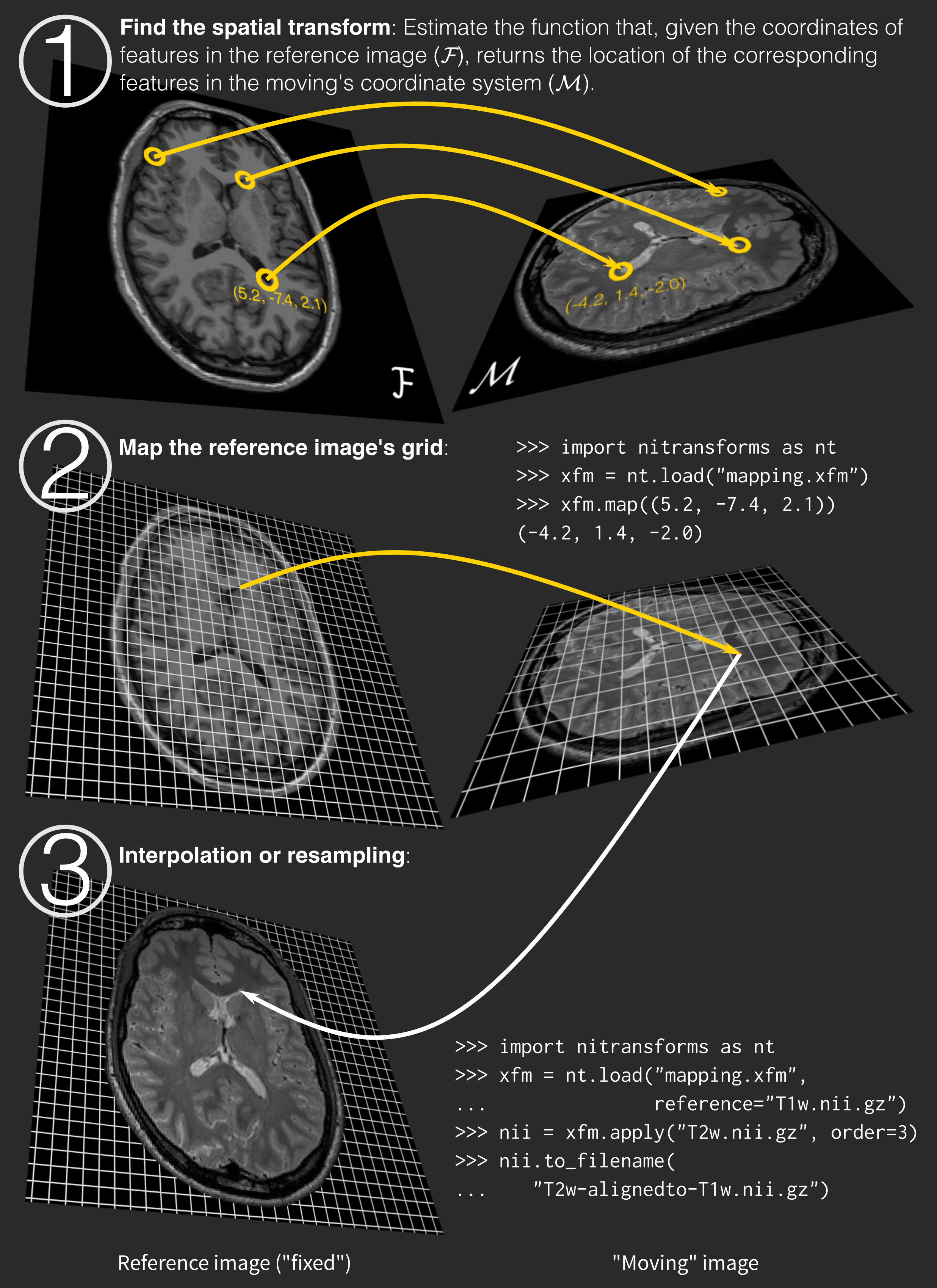
NiTransforms (open-access pre-print here) is an ongoing project to bring a compatibility layer into NiBabel between the many transform file formats generated by neuroimaging packages. We will be using NiTransforms to apply these transforms we estimate with ANTs – effectively resampling moving images into their reference’s grid.
To read a transform produced by ANTs with NiTransforms, we use the following piece of code:
import nitransforms as nt

itk_xform = nt.io.itk.ITKLinearTransform.from_filename(result.outputs.forward_transforms[0])
matrix = itk_xform.to_ras(reference=fixed_path, moving=moving_path)
matrix
array([[ 0.9974625 , -0.00625172,  0.00114571,  0.07182863],
       [ 0.00605242,  0.99567397, -0.00871013, -0.10887415],
       [-0.00233421,  0.02094301,  0.99652648, -0.85758593],
       [ 0.        ,  0.        ,  0.        ,  1.        ]])
Resampling an image requires two pieces of information: the reference image (which provides the new grid where we want to have the data) and the moving image which contains the actual data we are interested in:
xfm = nt.linear.Affine(matrix)
xfm.reference = fixed_path
resampled = xfm.apply(moving_path)
resampled.to_filename(tempdir / "resampled-nitransforms.nii.gz")

display(
    fixed_path,
    tempdir / "resampled-nitransforms.nii.gz",
    fixed_label="Predicted",
    moving_label="Aligned (nitransforms)",
);
Exercise
Use the display() function to visualize the image aligned as generated by ANTs vs. that generated by NiTransforms – they should be aligned!.
Solution